Hash-Based Indexing
Database Systems - Unit III
Dr. Mohsin Dar
Assistant Professor
Cloud & Software Operations Cluster
UPES - MTech First Semester
Introduction to Hash-Based Indexing
What is Hashing?
- Hashing is a technique that uses a hash function to compute the address of a data record based on its search key value
- Provides O(1) average time complexity for search, insert, and delete operations
- Alternative to tree-based indexing (B-Trees, B+ Trees)
Key Components
- Hash Function h(k): Maps search key k to a bucket address
- Buckets: Storage units that hold one or more records
- Collision: When multiple keys hash to the same bucket
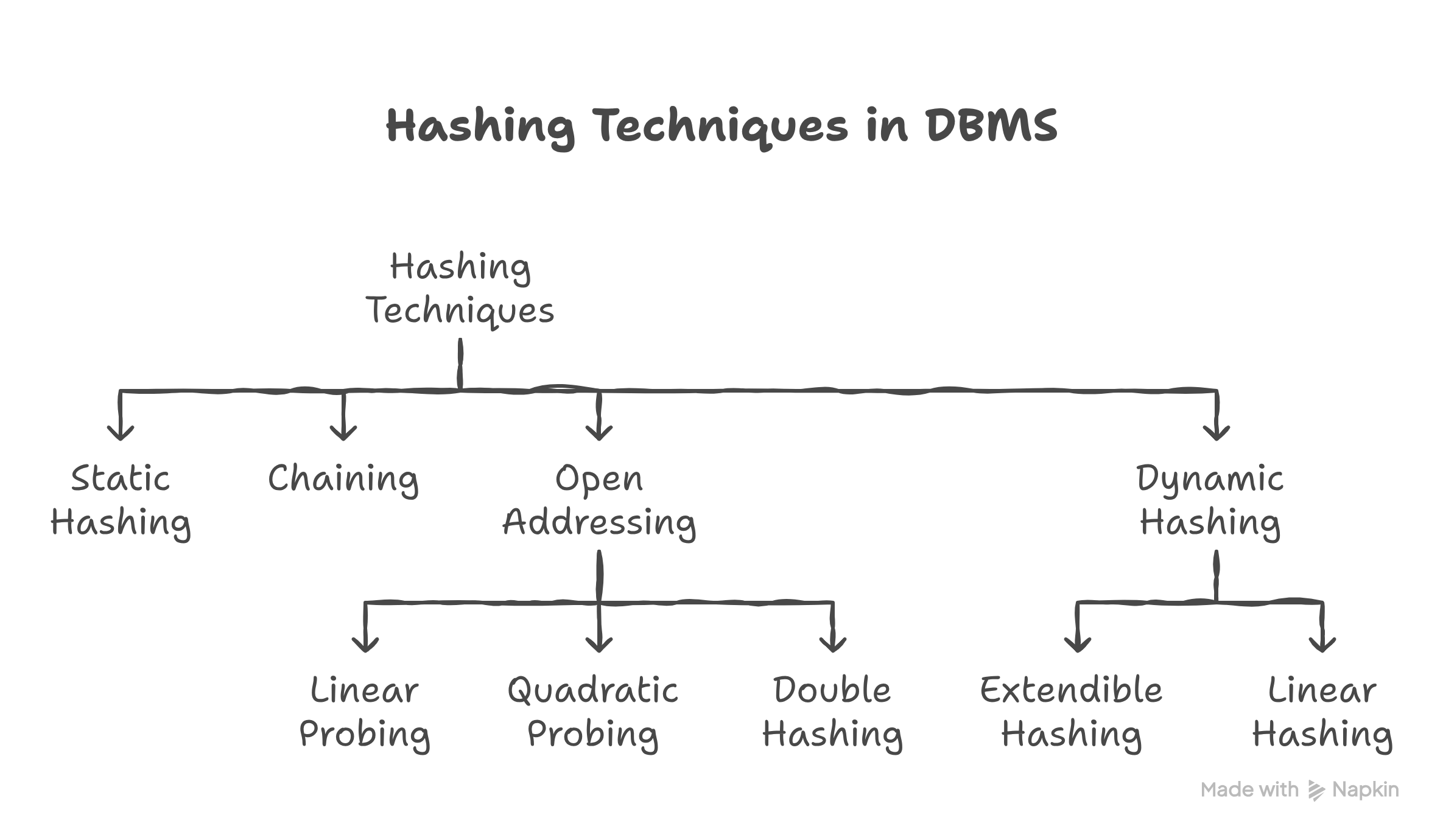
Figure: Visual representation of hashing process
Hash Function Visualization
Example: h(k) = k mod 5
Keys: 12, 17, 23, 8, 31, 19
Static Hashing
Definition
- Fixed number of buckets allocated at creation time
- Hash function maps keys to a fixed range of bucket addresses
- Simplest form of hash-based indexing
Characteristics
- Fixed Structure: Number of buckets (N) remains constant
- Overflow Handling: Uses overflow buckets/chains for collisions
- Performance: Degrades when load factor increases significantly
- Simple implementation
- Fast access when properly configured
- Predictable memory usage
Problems with Static Hashing
Major Limitations:
- Database Growth: Performance degrades as more records are added beyond initial capacity
- Long Overflow Chains: Multiple collisions create linked lists, degrading to O(n) search time
- Fixed Allocation: Cannot dynamically adjust to changing data volumes
- Space Wastage: Pre-allocating too many buckets wastes space; too few causes overflow
Solution Needed:
Dynamic hashing techniques that can grow and shrink based on the number of records
Extendable Hashing & Linear Hashing
Extendable Hashing
Concept
- Dynamic hashing technique that allows the hash structure to grow and shrink dynamically
- Uses a directory (lookup table) that can double in size when needed
- Based on binary representation of hash values
Key Components
- Global Depth (d): Number of bits used from the hash value for directory indexing
- Local Depth (d'): Number of bits used for a specific bucket
- Directory: Array of 2d bucket pointers
- Buckets: Store actual data records
Relationship
Local Depth ≤ Global Depth for all buckets
Extendable Hashing Structure
Example Structure (Global Depth = 2)
Extendable Hashing: Operations
Search Operation
2. Use first d bits to index into directory
3. Follow pointer to appropriate bucket
4. Search sequentially within bucket
Insert Operation
2. If bucket has space: Insert record
3. If bucket is full:
a) If local depth < global depth: Split bucket
b) If local depth = global depth: Double directory, then split bucket
4. Redistribute records based on additional bit
Delete Operation
2. If bucket becomes empty, merge with sibling bucket
3. Reduce local depth if appropriate
4. Halve directory if possible (all local depths < global depth)
Extendable Hashing: Insert Example
Scenario: Inserting key 20 causing bucket split
Before Insert (d=2)
Problem: Inserting 20 (10100) → ends with "00"
Bucket A is full!
After Split (d=3)
Solution: Global depth = local depth
→ Double directory (d=3)
→ Split bucket using 3rd bit
Extendible Hashing: Student Names Example
Student Names & Hashes
| Name | First Letter | Hash (binary) |
|---|---|---|
| Arun | A | 000 |
| Aditi | A | 001 |
| Aman | A | 010 |
| Bharat | B | 100 |
| Bina | B | 101 |
Step 1-2: Initial Setup (GD=1)
Step 3: After Inserting Arun, Aditi
Aditi (001) is added to B0
Step 4-6: Directory Doubling (GD=2)
Aman (010) causes split
Final State (After All Insertions)
Key: GD=2 (Global Depth), LD=Local Depth
Linear Hashing
Concept
- Dynamic hashing that grows one bucket at a time in a linear fashion
- No directory required - more space efficient than extendable hashing
- Uses multiple hash functions based on level
Key Components
- Level (L): Current round of splitting
- Next (N): Pointer to next bucket to split
- Hash Functions: hL(k) and hL+1(k)
- Split Threshold: Based on load factor
hL+1(k) = k mod (2L+1 × N0)
where N0 = initial number of buckets
Linear Hashing: How It Works
Split Trigger
- Split occurs when load factor exceeds threshold (typically 0.7-0.8)
- Bucket that caused overflow may NOT be the one that splits!
- Split follows round-robin order from bucket 0
Split Process
2. Create new bucket at end of file
3. Redistribute records from bucket N using hL+1
4. Increment Next pointer
5. If all buckets in current level split → increment Level (L)
Search Strategy
2. If B < Next: Bucket already split, use hL+1(k)
3. If B ≥ Next: Bucket not yet split, use hL(k)
Linear Hashing: Example
Initial State: L=0, N=0, N0=4
Hash Functions:
h0(k) = k mod 4
h1(k) = k mod 8
Extendable vs Linear Hashing
| Aspect | Extendable Hashing | Linear Hashing |
|---|---|---|
| Directory | Required (can double in size) | Not required |
| Growth Pattern | Exponential (doubles) | Linear (one bucket at a time) |
| Split Trigger | Bucket overflow | Load factor threshold |
| Which Bucket Splits | Overflowing bucket | Next in round-robin order |
| Space Overhead | Directory space overhead | Minimal overhead |
| Performance | 1-2 disk accesses | 1-2 disk accesses + overflow |
| Complexity | Moderate | Higher (multiple hash functions) |
Hash-Based Indexing: Trade-offs
✓ Advantages of Hash-Based Indexing
- Fast Access: O(1) average case for equality searches
- Simple Implementation: Straightforward hash function logic
- Uniform Distribution: Good hash functions distribute data evenly
- Dynamic Growth: Extendable and Linear hashing adapt to data size
- No Reordering: Records don't need to maintain sorted order
✗ Disadvantages of Hash-Based Indexing
- No Range Queries: Cannot efficiently support range searches (e.g., age > 25)
- No Ordering: Cannot retrieve records in sorted order
- Collision Overhead: Performance degrades with poor hash functions
- Space Wastage: Empty buckets in static hashing
- Complex Maintenance: Dynamic hashing requires split/merge operations
When to Use: Hash vs Tree Indexing
Use Hash-Based Indexing When:
- Queries are primarily equality searches (exact match)
- No requirement for ordered retrieval or sorting
- No range queries needed
- Fast single-record access is critical
- Example:
SELECT * FROM Students WHERE StudentID = 12345
Use Tree-Based Indexing (B+Tree) When:
- Need to support range queries (e.g., salary BETWEEN 50000 AND 80000)
- Ordered traversal required (e.g., ORDER BY)
- Prefix matching (e.g., name LIKE 'John%')
- Multi-attribute indexing with ordering
- Example:
SELECT * FROM Employees WHERE Age > 30 AND Age < 50
Collision Resolution Techniques
1. Chaining (Separate Chaining)
- Each bucket maintains a linked list of all records that hash to it
- Most common in database systems
- Allows unlimited records per bucket (limited by memory)
2. Open Addressing
- Linear Probing: Search sequentially for next empty slot
- Quadratic Probing: Use quadratic function to find next slot
- Double Hashing: Use second hash function for probing
- Less common in database systems due to deletion complexity
3. Overflow Buckets
- Primary bucket points to overflow area when full
- Used in static hashing
- Can create long overflow chains affecting performance
Performance Analysis
Time Complexity Comparison
| Operation | Hash Index | B+Tree Index |
|---|---|---|
| Equality Search | O(1) average | O(log n) |
| Range Search | O(n) - Not supported | O(log n + k) |
| Insert | O(1) average | O(log n) |
| Delete | O(1) average | O(log n) |
| Ordered Traversal | O(n log n) - Not supported | O(n) |
Space Complexity
- Static Hashing: O(N) where N = number of buckets
- Extendable Hashing: O(2d) for directory + O(N) for buckets
- Linear Hashing: O(N) where N = current number of buckets
- B+Tree: O(N) where N = number of nodes
Real-World Applications
Database Systems Using Hash Indexing
- PostgreSQL: Hash indexes for equality comparisons
- Oracle: Hash clusters for frequently accessed tables
- MySQL: Hash indexes in MEMORY storage engine
- NoSQL Databases: DynamoDB, Cassandra use consistent hashing
Common Use Cases
Best Practices & Design Guidelines
Choosing Hash Function
- Select hash function that provides uniform distribution
- Avoid functions that create clustering
- Common choices: Division method, Multiplication method, Universal hashing
Configuration Guidelines
When NOT to Use Hashing
- Primary access pattern involves range queries
- Need sorted output frequently
- Partial key searches required
- Data has high skew (non-uniform distribution)
Summary: Hash-Based Indexing
Key Takeaways
- Range Query Support - Ordered Access
Understanding the trade-offs is key to choosing the right indexing technique!
Questions?
Hash-Based Indexing
Dr. Mohsin Dar
Assistant Professor
SOCS | UPES
Next: Tree-Based Indexing Deep Dive